A Simple Example
a-simple-example.Rmd
# set CRAN mirror
options(repos = c(CRAN = "https://cran.rstudio.com"))

# Get rid of memory limits -----------------------------------------------------
options(future.globals.maxSize = 1 * 1024^4) # Allow up to 1 TB for globals

# Install Libraries ------------------------------------------------------------

# Here we list all the packages we will need for this whole process
# We'll also use this in our works cited page.
PKG <- c(
  "surveyresamplr",
  "dplyr",
  "tidyr",
  "purrr",
  "ggplot2",
  "future.callr",
  "flextable",
  "sdmTMB"
)

pkg_install <- function(p) {
  if (!require(p, character.only = TRUE)) {
    install.packages(p)
  }
  require(p, character.only = TRUE)
}
base::lapply(unique(PKG), pkg_install)
#> Loading required package: surveyresamplr
#> Loading required package: dplyr
#>
#> Attaching package: 'dplyr'
#> The following objects are masked from 'package:stats':
#>
#>     filter, lag
#> The following objects are masked from 'package:base':
#>
#>     intersect, setdiff, setequal, union
#> Loading required package: tidyr
#> Loading required package: purrr
#> Loading required package: ggplot2
#> Loading required package: future.callr
#> Loading required package: future
#> Loading required package: flextable
#>
#> Attaching package: 'flextable'
#> The following object is masked from 'package:purrr':
#>
#>     compose
#> Loading required package: sdmTMB
#> [[1]]
#> [1] TRUE
#>
#> [[2]]
#> [1] TRUE
#>
#> [[3]]
#> [1] TRUE
#>
#> [[4]]
#> [1] TRUE
#>
#> [[5]]
#> [1] TRUE
#>
#> [[6]]
#> [1] TRUE
#>
#> [[7]]
#> [1] TRUE
#>
#> [[8]]
#> [1] TRUE

# Set directories --------------------------------------------------------------
wd <- paste0(here::here(), "/vignettes/")
dir_out <- paste0(wd, "output/")
dir_final <- paste0(dir_out, "CA_0results/")
Test Species List
Then we define our species and model list. In this simple example, we’ll assess a model for eastern Bering Sea (EBS) walleye pollock (Gadus chalcogrammus) from 2015-present, using data collected by the Alaska Fisheries Science Center.
Walleye pollock are fairly well distributed across the area, very common in the area, and very economically important, so this will be a great species to start testing these models with.
spp_list <- data.frame(
  srvy = "EBS",
  common_name = "walleye pollock",
  file_name = "simple_walleye_pollock",
  species_code = as.character(21740),
  filter_lat_lt = NA,
  filter_lat_gt = NA,
  filter_depth = NA,
  model_fn = "total_catch_wt_kg ~ 0 + factor(year)",
  model_family = "delta_gamma",
  model_anisotropy = TRUE,
  model_spatiotemporal = "iid, iid"
)
Pull in data
Some example data is included in the R package for examples like this. We’ll need
- Zero-filled catch data from the survey to use for developing the model and
- an extrapolation grid that you can replicate across years for your prediction matrix. Note that if your model models over depth (as with this model) your prediction grid will also need to have a depth field.
Use ?surveyresamplr::noaa_afsc_catch and
?surveyresamplr::noaa_afsc_ebs_pred_grid_depth) to learn
more about these data sources. In the meantime, this is what these
resources look like:
# ?surveyresamplr::noaa_afsc_catch

head(surveyresamplr::noaa_afsc_catch) |>
  flextable::flextable()
srvy |
trawlid |
common_name |
species_code |
total_catch_numbers |
total_catch_wt_kg |
cpue_kgkm2 |
latitude_dd |
longitude_dd |
year |
bottom_temperature_c |
depth_m |
|---|---|---|---|---|---|---|---|---|---|---|---|
BSS |
1,225,491 |
walleye pollock |
21,740 |
40 |
52.360 |
1,360.96434 |
54.57648 |
-166.5989 |
2,004 |
3.9 |
413 |
BSS |
1,225,492 |
walleye pollock |
21,740 |
1 |
0.558 |
14.18031 |
55.12762 |
-167.8108 |
2,004 |
3.8 |
430 |
BSS |
1,225,493 |
walleye pollock |
21,740 |
54.94091 |
-167.7837 |
2,004 |
2.8 |
1,016 |
|||
BSS |
1,225,494 |
walleye pollock |
21,740 |
9 |
10.090 |
277.73894 |
58.39780 |
-174.4882 |
2,004 |
3.9 |
340 |
BSS |
1,225,495 |
walleye pollock |
21,740 |
58.50877 |
-174.8404 |
2,004 |
2.8 |
1,024 |
|||
BSS |
1,225,496 |
walleye pollock |
21,740 |
48 |
72.730 |
2,083.51674 |
58.55886 |
-174.6119 |
2,004 |
3.9 |
324 |
dat <- surveyresamplr::noaa_afsc_catch |>
  dplyr::filter(year %in% 2023:2024 &
    srvy %in% c("EBS") &
    species_code == 21740)

ggplot2::ggplot(
  data = dat |> dplyr::filter(cpue_kgkm2 != 0),
  mapping = aes(
    x = longitude_dd,
    y = latitude_dd,
    size = cpue_kgkm2
  )
) +
  ggplot2::geom_point(alpha = .75) +
  ggplot2::geom_point(
    data = dat |> dplyr::filter(cpue_kgkm2 %in% c(0, NA)),
    color = "red",
    shape = 17,
    alpha = .75,
    size = 3
  ) +
  ggplot2::xlab("Longitude °W") +
  ggplot2::ylab("Latitude °N") +
  ggplot2::ggtitle(
    label = "CPUE (kg/km^2) of walleye pollock (Weight CPUE; kg/km2)",
    subtitle = "AFSC Eastern Bering Sea bottom trawl survey"
  ) +
  ggplot2::scale_size_continuous(name = "Weight (kg)") +
  ggplot2::facet_wrap(facets = vars(year)) +
  ggplot2::theme_bw()
CPUE (kg/km^2) of walleye pollock (Weight CPUE; kg/km2) from 2023 and 2024 in the EBS survey.
# ?surveyresamplr::noaa_afsc_ebs_pred_grid_depth

head(surveyresamplr::noaa_afsc_ebs_pred_grid_depth) |>
  flextable::flextable()
depth_m |
latitude_dd |
longitude_dd |
area_km2 |
stratum |
pass |
srvy |
|---|---|---|---|---|---|---|
93 |
62.12637 |
-176.1836 |
2.449159 |
82 |
1 |
EBS |
92 |
62.14212 |
-176.1320 |
9.298534 |
82 |
1 |
EBS |
92 |
62.15210 |
-176.0715 |
9.749166 |
82 |
1 |
EBS |
92 |
62.15774 |
-176.0025 |
5.383834 |
82 |
1 |
EBS |
92 |
62.16243 |
-175.9448 |
1.173734 |
82 |
1 |
EBS |
93 |
62.07334 |
-176.2894 |
1.525663 |
82 |
1 |
EBS |
ggplot2::ggplot(
  data = surveyresamplr::noaa_afsc_ebs_pred_grid_depth,
  mapping = aes(
    x = longitude_dd,
    y = latitude_dd,
    color = depth_m
  )
) +
  ggplot2::geom_point(
    alpha = .5,
    size = .5
  ) +
  ggplot2::xlab("Longitude °W") +
  ggplot2::ylab("Latitude °N") +
  ggplot2::ggtitle(
    label = "Prediction Grid",
    subtitle = "AFSC Eastern Bering Sea bottom trawl survey"
  ) +
  ggplot2::scale_color_gradient(name = "Depth (m)") +
  ggplot2::theme_bw()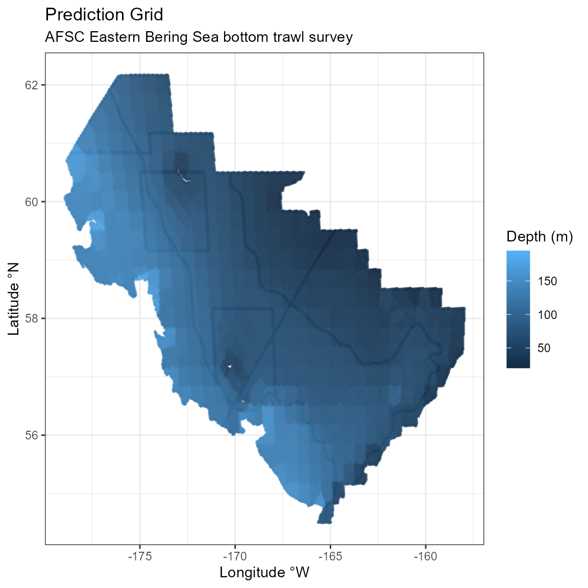
Prediction grid for the EBS survey.
Here we load the data for the model run, cropping it to the data we would like to include (the EBS survey and years greater than 2010) and replicating the the prediction grid across the years in the catch data.
### Load survey data -----------------------------------------------------------

catch <- surveyresamplr::noaa_afsc_catch |>
  dplyr::filter(srvy == "EBS") |>
  dplyr::filter(year >= 2015)

### Load grid data -------------------------------------------------------------

grid_yrs <- sdmTMB::replicate_df(
  dat = surveyresamplr::noaa_afsc_ebs_pred_grid_depth,
  time_name = "year",
  time_values = unique(catch$year)
)
Now you’ll notice the year column has been added, repeated with all of the years in the catch data.
depth_m |
latitude_dd |
longitude_dd |
area_km2 |
stratum |
pass |
srvy |
year |
|---|---|---|---|---|---|---|---|
93 |
62.12637 |
-176.1836 |
2.449159 |
82 |
1 |
EBS |
2,022 |
92 |
62.14212 |
-176.1320 |
9.298534 |
82 |
1 |
EBS |
2,022 |
92 |
62.15210 |
-176.0715 |
9.749166 |
82 |
1 |
EBS |
2,022 |
92 |
62.15774 |
-176.0025 |
5.383834 |
82 |
1 |
EBS |
2,022 |
92 |
62.16243 |
-175.9448 |
1.173734 |
82 |
1 |
EBS |
2,022 |
93 |
62.07334 |
-176.2894 |
1.525663 |
82 |
1 |
EBS |
2,022 |
Set variables. This… requires more description.
seq(from = seq_from, to = seq_to, by = seq_by)
tot_dataframes = effort x replicates - (replicates - 1). TOLEDO: is this hard and fast?
srvy <- "EBS"
seq_from <- 0.50
seq_to <- 1.0
seq_by <- 0.25
tot_dataframes <- 3
replicate_num <- 7
Set directories
wd <- paste0(here::here(), "/vignettes/")
dir_out <- paste0(wd, "output/")
dir_final <- paste0(dir_out, "EBS_simple_0results/")
dir.create(dir_final, showWarnings = FALSE)
crs_latlon <- "+proj=longlat +datum=WGS84" # decimal degrees
Run resampling models
TOLDEO: explain why purrr::map is important, what the
sink files are for.
start.time <- Sys.time()
purrr::map(
  1:nrow(spp_list),
  ~ clean_and_resample(
    spp_list[.x, ],
    catch, seq_from, seq_to, seq_by,
    tot_dataframes, replicate_num, grid_yrs, dir_out
  )
)
write.csv(x = data.frame(time = as.numeric(Sys.time() - start.time), units = units(Sys.time() - start.time)), file = paste0(dir_final, srvy, "_simple_time.csv"))
a <- read.csv(file = paste0(dir_final, srvy, "_simple_time.csv"))
print(paste0("Time difference of ", round(a$time, 2), " ", a$units))
#> [1] "Time difference of 59.84 min"
# EBS walleye pollock
# ...Starting parallel SDM processing
#
# ...05_1
#
# This mesh has > 1000 vertices. Mesh complexity has the single largest influence on fitting speed. Consider whether you require a mesh this complex, especially for initial model exploration.
# Check `your_mesh$mesh$n` to view the number of vertices.Warning: The model may not have converged: non-positive-definite Hessian matrix.Warning: The model may not have converged: non-positive-definite Hessian matrix.Warning: NaNs producedWarning: NaNs producedWarning: NaNs producedWarning: NaNs producedWarning: NaNs producedWarning: NaNs producedWarning: NaNs producedWarning: NaNs produced✔ Non-linear minimizer suggests successful convergence
# ✖ Non-positive-definite Hessian matrix: model may not have converged
# ℹ Try simplifying the model, adjusting the mesh, or adding priors
#
# ✔ No extreme or very small eigenvalues detected
# ✔ No gradients with respect to fixed effects are >= 0.001
# Warning: NaNs producedWarning: NaNs producedWarning: NaNs producedWarning: NaNs produced✔ No fixed-effect standard errors are NA
# Warning: NaNs producedWarning: NaNs producedWarning: NaNs producedWarning: NaNs produced✖ `b_j` standard error may be large
# ℹ Try simplifying the model, adjusting the mesh, or adding priors
#
# ✖ `ln_kappa` standard error may be large
# ℹ `ln_kappa` is an internal parameter affecting `range`
# ℹ `range` is the distance at which data are effectively independent
# ℹ Try simplifying the model, adjusting the mesh, or adding priors
#
# Warning: NaNs producedWarning: NaNs producedWarning: NaNs producedWarning: NaNs producedWarning: NaNs producedWarning: NaNs producedWarning: NaNs producedWarning: NaNs producedWarning: NaNs producedWarning: NaNs producedWarning: NaNs producedWarning: NaNs producedWarning: NaNs producedWarning: NaNs producedWarning: NaNs producedWarning: NaNs produced✔ No sigma parameters are < 0.01
# ✔ No sigma parameters are > 100
# ✔ Range parameters don't look unreasonably large
#
# ...05_2
#
# This mesh has > 1000 vertices. Mesh complexity has the single largest influence on fitting speed. Consider whether you require a mesh this complex, especially for initial model exploration.
# Check `your_mesh$mesh$n` to view the number of vertices.Warning: NaNs producedWarning: The model may not have converged: non-positive-definite Hessian matrix.Warning: NaNs producedWarning: The model may not have converged: non-positive-definite Hessian matrix.Warning: NaNs producedWarning: NaNs producedWarning: NaNs producedWarning: NaNs producedWarning: NaNs producedWarning: NaNs producedWarning: NaNs producedWarning: NaNs produced✔ Non-linear minimizer suggests successful convergence
# ✖ Non-positive-definite Hessian matrix: model may not have converged
# ℹ Try simplifying the model, adjusting the mesh, or adding priors
#
# ✔ No extreme or very small eigenvalues detected
# ✖ `b_j2` gradient > 0.001
# ℹ See ?run_extra_optimization(), standardize covariates, and/or simplify the model
#
# ✖ `ln_tau_E` gradient > 0.001
# ℹ See ?run_extra_optimization(), standardize covariates, and/or simplify the model
#
# ✖ `ln_kappa` gradient > 0.001
# ℹ See ?run_extra_optimization(), standardize covariates, and/or simplify the model
#
# ✖ `ln_phi` gradient > 0.001
# ℹ See ?run_extra_optimization(), standardize covariates, and/or simplify the model
#
# Warning: NaNs producedWarning: NaNs producedWarning: NaNs producedWarning: NaNs produced✔ No fixed-effect standard errors are NA
# Warning: NaNs producedWarning: NaNs producedWarning: NaNs producedWarning: NaNs produced✖ `b_j` standard error may be large
# ℹ Try simplifying the model, adjusting the mesh, or adding priors
#
# Warning: NaNs producedWarning: NaNs producedWarning: NaNs producedWarning: NaNs producedWarning: NaNs producedWarning: NaNs producedWarning: NaNs producedWarning: NaNs producedWarning: NaNs producedWarning: NaNs producedWarning: NaNs producedWarning: NaNs producedWarning: NaNs producedWarning: NaNs producedWarning: NaNs producedWarning: NaNs produced✔ No sigma parameters are < 0.01
# ✔ No sigma parameters are > 100
# ✔ Range parameters don't look unreasonably large
#
# ...05_3
#
# This mesh has > 1000 vertices. Mesh complexity has the single largest influence on fitting speed. Consider whether you require a mesh this complex, especially for initial model exploration.
# Check `your_mesh$mesh$n` to view the number of vertices.Warning: NaNs producedWarning: The model may not have converged: non-positive-definite Hessian matrix.Warning: NaNs producedWarning: The model may not have converged: non-positive-definite Hessian matrix.Warning: NaNs producedWarning: NaNs producedWarning: NaNs producedWarning: NaNs producedWarning: NaNs producedWarning: NaNs producedWarning: NaNs producedWarning: NaNs produced✔ Non-linear minimizer suggests successful convergence
# ✖ Non-positive-definite Hessian matrix: model may not have converged
# ℹ Try simplifying the model, adjusting the mesh, or adding priors
#
# ✔ No extreme or very small eigenvalues detected
# ✖ `b_j2` gradient > 0.001
# ℹ See ?run_extra_optimization(), standardize covariates, and/or simplify the model
#
# ✖ `b_j2` gradient > 0.001
# ℹ See ?run_extra_optimization(), standardize covariates, and/or simplify the model
#
# ✖ `ln_tau_E` gradient > 0.001
# ℹ See ?run_extra_optimization(), standardize covariates, and/or simplify the model
#
# ✖ `ln_kappa` gradient > 0.001
# ℹ See ?run_extra_optimization(), standardize covariates, and/or simplify the model
#
# Warning: NaNs producedWarning: NaNs producedWarning: NaNs producedWarning: NaNs produced✔ No fixed-effect standard errors are NA
# Warning: NaNs producedWarning: NaNs producedWarning: NaNs producedWarning: NaNs produced✖ `b_j` standard error may be large
# ℹ Try simplifying the model, adjusting the mesh, or adding priors
#
# Warning: NaNs producedWarning: NaNs producedWarning: NaNs producedWarning: NaNs producedWarning: NaNs producedWarning: NaNs producedWarning: NaNs producedWarning: NaNs producedWarning: NaNs producedWarning: NaNs producedWarning: NaNs producedWarning: NaNs producedWarning: NaNs producedWarning: NaNs producedWarning: NaNs producedWarning: NaNs produced✔ No sigma parameters are < 0.01
# ✔ No sigma parameters are > 100
# ✔ Range parameters don't look unreasonably large
# ...Parallel SDM processing complete
out <- plot_results(srvy = paste0(srvy, "_simple"), dir_out = dir_out, dir_final = dir_final)
out$plots
#> $index_boxplot_log_biomass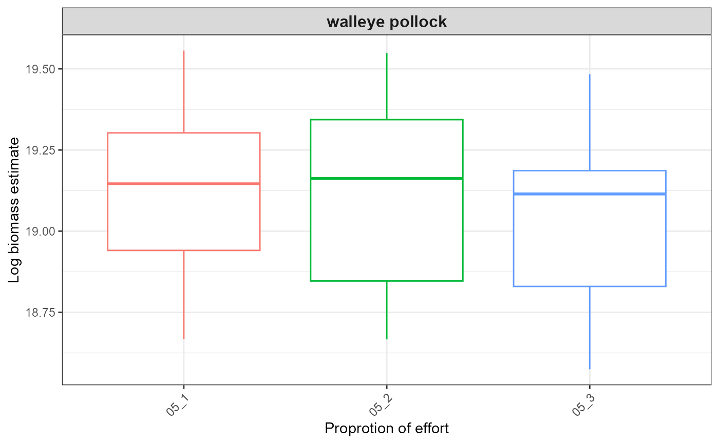
#>
#> $index_boxplot_log_biomass_SE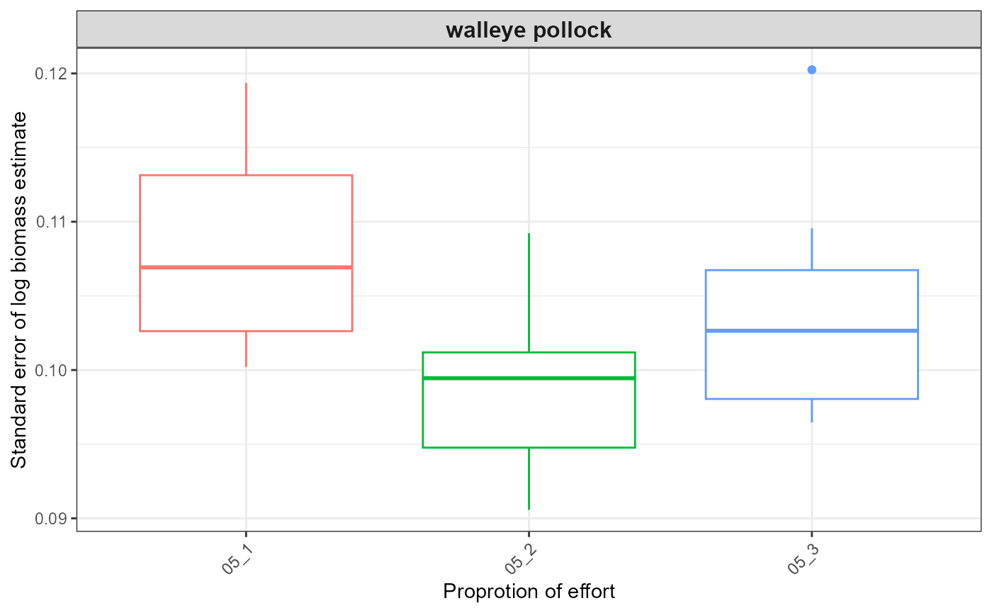
#>
#> $index_boxplot_biomass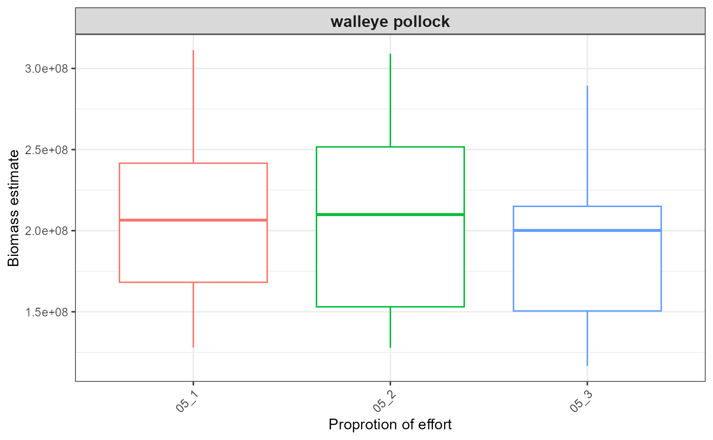
#>
#> $index_timeseries_biomass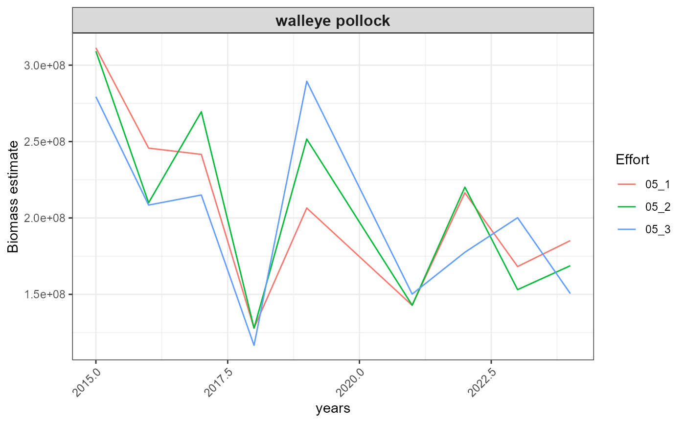
Parameter output:
i <- 1
print(names(out$tables)[i])
#> [1] "fit_df"
head(out$tables[i][[1]]) |>
  flextable::flextable()
X.5 |
X.4 |
X.3 |
X.2 |
X.1 |
X |
srvy |
common_name |
file_name |
species_code |
filter_lat_lt |
filter_lat_gt |
filter_depth |
model_fn |
model_family |
model_anisotropy |
model_spatiotemporal |
effort |
term |
estimate |
std.error |
conf.low |
conf.high |
|---|---|---|---|---|---|---|---|---|---|---|---|---|---|---|---|---|---|---|---|---|---|---|
1 |
1 |
1 |
1 |
1 |
1 |
EBS |
walleye pollock |
walleye_pollock_test |
21,740 |
total_catch_wt_kg ~ 0 + factor(year) |
delta_gamma |
TRUE |
iid, iid |
05_1 |
factor(year)2015 |
19.77117 |
1,391.123 |
-2,706.781 |
2,746.323 |
|||
2 |
2 |
2 |
2 |
2 |
2 |
EBS |
walleye pollock |
walleye_pollock_test |
21,740 |
total_catch_wt_kg ~ 0 + factor(year) |
delta_gamma |
TRUE |
iid, iid |
05_1 |
factor(year)2016 |
19.90634 |
1,384.990 |
-2,694.625 |
2,734.437 |
|||
3 |
3 |
3 |
3 |
3 |
3 |
EBS |
walleye pollock |
walleye_pollock_test |
21,740 |
total_catch_wt_kg ~ 0 + factor(year) |
delta_gamma |
TRUE |
iid, iid |
05_1 |
factor(year)2017 |
19.86007 |
1,340.321 |
-2,607.120 |
2,646.840 |
|||
4 |
4 |
4 |
4 |
4 |
4 |
EBS |
walleye pollock |
walleye_pollock_test |
21,740 |
total_catch_wt_kg ~ 0 + factor(year) |
delta_gamma |
TRUE |
iid, iid |
05_1 |
factor(year)2018 |
19.80071 |
1,454.167 |
-2,830.315 |
2,869.916 |
|||
5 |
5 |
5 |
5 |
5 |
5 |
EBS |
walleye pollock |
walleye_pollock_test |
21,740 |
total_catch_wt_kg ~ 0 + factor(year) |
delta_gamma |
TRUE |
iid, iid |
05_1 |
factor(year)2019 |
20.11844 |
1,272.466 |
-2,473.869 |
2,514.106 |
|||
6 |
6 |
6 |
6 |
6 |
6 |
EBS |
walleye pollock |
walleye_pollock_test |
21,740 |
total_catch_wt_kg ~ 0 + factor(year) |
delta_gamma |
TRUE |
iid, iid |
05_1 |
factor(year)2021 |
19.71943 |
1,278.253 |
-2,485.611 |
2,525.050 |
i <- 1 + i
print(names(out$tables)[i])
#> [1] "fit_pars"
head(out$tables[i][[1]]) |>
  flextable::flextable()
X.5 |
X.4 |
X.3 |
X.2 |
X.1 |
X |
srvy |
common_name |
file_name |
species_code |
filter_lat_lt |
filter_lat_gt |
filter_depth |
model_fn |
model_family |
model_anisotropy |
model_spatiotemporal |
effort |
term |
estimate |
std.error |
conf.low |
conf.high |
|---|---|---|---|---|---|---|---|---|---|---|---|---|---|---|---|---|---|---|---|---|---|---|
1 |
1 |
1 |
1 |
1 |
1 |
EBS |
walleye pollock |
walleye_pollock_test |
21,740 |
total_catch_wt_kg ~ 0 + factor(year) |
delta_gamma |
TRUE |
iid, iid |
05_1 |
range |
3.7298099 |
3,393.6903 |
0 |
Inf |
|||
2 |
2 |
2 |
2 |
2 |
2 |
EBS |
walleye pollock |
walleye_pollock_test |
21,740 |
total_catch_wt_kg ~ 0 + factor(year) |
delta_gamma |
TRUE |
iid, iid |
05_1 |
sigma_O |
0.1812892 |
140.5073 |
0 |
Inf |
|||
3 |
3 |
3 |
3 |
3 |
3 |
EBS |
walleye pollock |
walleye_pollock_test |
21,740 |
total_catch_wt_kg ~ 0 + factor(year) |
delta_gamma |
TRUE |
iid, iid |
05_1 |
sigma_E |
0.3717503 |
336.2267 |
0 |
Inf |
|||
4 |
4 |
4 |
4 |
4 |
EBS |
walleye pollock |
walleye_pollock_test |
21,740 |
total_catch_wt_kg ~ 0 + factor(year) |
delta_gamma |
TRUE |
iid, iid |
05_2 |
range |
2.8284007 |
|||||||
5 |
5 |
5 |
5 |
5 |
EBS |
walleye pollock |
walleye_pollock_test |
21,740 |
total_catch_wt_kg ~ 0 + factor(year) |
delta_gamma |
TRUE |
iid, iid |
05_2 |
sigma_O |
0.2820909 |
|||||||
6 |
6 |
6 |
6 |
6 |
EBS |
walleye pollock |
walleye_pollock_test |
21,740 |
total_catch_wt_kg ~ 0 + factor(year) |
delta_gamma |
TRUE |
iid, iid |
05_2 |
sigma_E |
0.2820909 |
i <- 1 + i
print(names(out$tables)[i])
#> [1] "fit_check"
head(out$tables[i][[1]]) |>
  flextable::flextable()
X.5 |
X.4 |
X.3 |
X.2 |
X.1 |
X |
srvy |
common_name |
file_name |
species_code |
filter_lat_lt |
filter_lat_gt |
filter_depth |
model_fn |
model_family |
model_anisotropy |
model_spatiotemporal |
effort |
hessian_ok |
eigen_values_ok |
nlminb_ok |
range_ok |
gradients_ok |
se_magnitude_ok |
se_na_ok |
sigmas_ok |
all_ok |
|---|---|---|---|---|---|---|---|---|---|---|---|---|---|---|---|---|---|---|---|---|---|---|---|---|---|---|
1 |
1 |
1 |
1 |
1 |
1 |
EBS |
walleye pollock |
walleye_pollock_test |
21,740 |
total_catch_wt_kg ~ 0 + factor(year) |
delta_gamma |
TRUE |
iid, iid |
05_1 |
FALSE |
TRUE |
TRUE |
TRUE |
TRUE |
FALSE |
TRUE |
TRUE |
FALSE |
|||
2 |
2 |
2 |
2 |
2 |
EBS |
walleye pollock |
walleye_pollock_test |
21,740 |
total_catch_wt_kg ~ 0 + factor(year) |
delta_gamma |
TRUE |
iid, iid |
05_2 |
FALSE |
TRUE |
TRUE |
TRUE |
FALSE |
FALSE |
TRUE |
TRUE |
FALSE |
||||
3 |
3 |
3 |
3 |
EBS |
walleye pollock |
walleye_pollock_test |
21,740 |
total_catch_wt_kg ~ 0 + factor(year) |
delta_gamma |
TRUE |
iid, iid |
05_3 |
FALSE |
TRUE |
TRUE |
TRUE |
FALSE |
FALSE |
TRUE |
TRUE |
FALSE |
|||||
4 |
4 |
4 |
EBS |
walleye pollock |
simple_walleye_pollock |
21,740 |
total_catch_wt_kg ~ 0 + factor(year) |
delta_gamma |
TRUE |
iid, iid |
05_1 |
FALSE |
TRUE |
TRUE |
TRUE |
TRUE |
FALSE |
TRUE |
TRUE |
FALSE |
||||||
5 |
5 |
EBS |
walleye pollock |
simple_walleye_pollock |
21,740 |
total_catch_wt_kg ~ 0 + factor(year) |
delta_gamma |
TRUE |
iid, iid |
05_2 |
FALSE |
TRUE |
TRUE |
TRUE |
FALSE |
FALSE |
TRUE |
TRUE |
FALSE |
|||||||
6 |
EBS |
walleye pollock |
simple_walleye_pollock |
21,740 |
total_catch_wt_kg ~ 0 + factor(year) |
delta_gamma |
TRUE |
iid, iid |
05_3 |
FALSE |
TRUE |
TRUE |
TRUE |
FALSE |
FALSE |
TRUE |
TRUE |
FALSE |
i <- 1 + i
print(names(out$tables)[i])
#> [1] "index"
head(out$tables[i][[1]]) |>
  flextable::flextable()
X.5 |
X.4 |
X.3 |
X.2 |
X.1 |
X |
srvy |
common_name |
file_name |
species_code |
filter_lat_lt |
filter_lat_gt |
filter_depth |
model_fn |
model_family |
model_anisotropy |
model_spatiotemporal |
effort |
year |
est |
lwr |
upr |
log_est |
se |
type |
|---|---|---|---|---|---|---|---|---|---|---|---|---|---|---|---|---|---|---|---|---|---|---|---|---|
1 |
1 |
1 |
1 |
1 |
1 |
EBS |
walleye pollock |
walleye_pollock_test |
21,740 |
total_catch_wt_kg ~ 0 + factor(year) |
delta_gamma |
TRUE |
iid, iid |
05_1 |
2,015 |
311,329,658 |
254,290,109 |
381,163,688 |
19.55636 |
0.1032552 |
index |
|||
2 |
2 |
2 |
2 |
2 |
2 |
EBS |
walleye pollock |
walleye_pollock_test |
21,740 |
total_catch_wt_kg ~ 0 + factor(year) |
delta_gamma |
TRUE |
iid, iid |
05_1 |
2,016 |
245,697,312 |
201,795,592 |
299,150,087 |
19.31961 |
0.1004330 |
index |
|||
3 |
3 |
3 |
3 |
3 |
3 |
EBS |
walleye pollock |
walleye_pollock_test |
21,740 |
total_catch_wt_kg ~ 0 + factor(year) |
delta_gamma |
TRUE |
iid, iid |
05_1 |
2,017 |
241,587,105 |
198,504,083 |
294,020,799 |
19.30274 |
0.1002163 |
index |
|||
4 |
4 |
4 |
4 |
4 |
4 |
EBS |
walleye pollock |
walleye_pollock_test |
21,740 |
total_catch_wt_kg ~ 0 + factor(year) |
delta_gamma |
TRUE |
iid, iid |
05_1 |
2,018 |
127,954,658 |
101,264,147 |
161,680,073 |
18.66719 |
0.1193611 |
index |
|||
5 |
5 |
5 |
5 |
5 |
5 |
EBS |
walleye pollock |
walleye_pollock_test |
21,740 |
total_catch_wt_kg ~ 0 + factor(year) |
delta_gamma |
TRUE |
iid, iid |
05_1 |
2,019 |
206,496,853 |
166,663,257 |
255,850,936 |
19.14580 |
0.1093438 |
index |
|||
6 |
6 |
6 |
6 |
6 |
6 |
EBS |
walleye pollock |
walleye_pollock_test |
21,740 |
total_catch_wt_kg ~ 0 + factor(year) |
delta_gamma |
TRUE |
iid, iid |
05_1 |
2,021 |
142,822,421 |
115,820,004 |
176,120,214 |
18.77711 |
0.1069228 |
index |