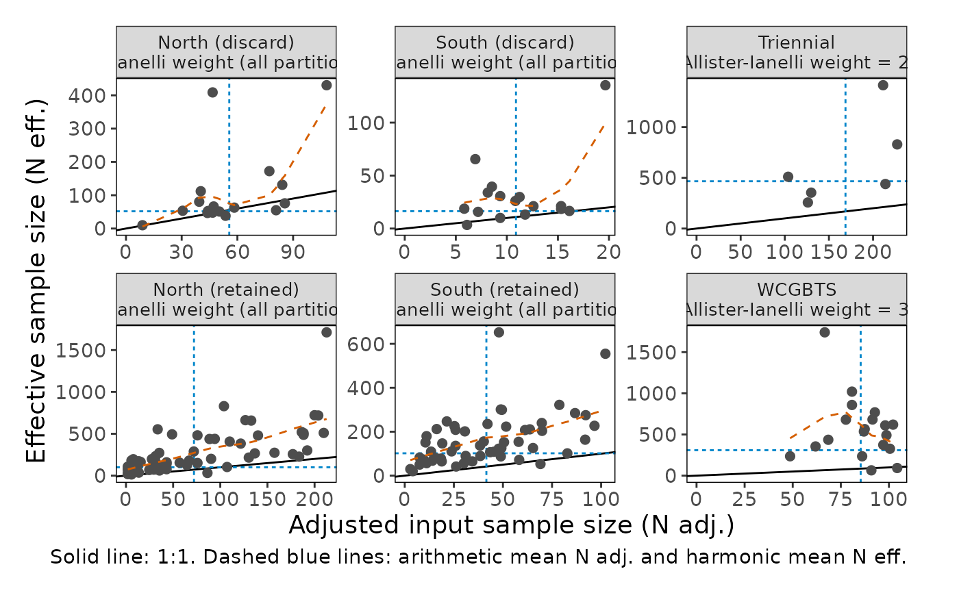
Plot input versus effective sample size of compositions
Source:R/plot_composition_diagnostics.R
plot_composition_samples.RdCompare the input (or adjusted input) sample size of each composition with its effective sample size, the sample size implied by how well the model fits the composition. This is the diagnostic behind the McAllister and Ianelli (1997) data weighting method.
plot_composition_samples(
  dat,
  comp_type = NULL,
  fleet = NULL,
  show_years = FALSE,
  ncol = NULL,
  direction = "v"
)
Arguments
- dat
A tibble returned from
convert_output()that contains composition data (see bigskate_lencomp), or composition data in any other format accepted byprepare_composition_data(). For Stock Synthesis output converted from a Report.sso file without compositions by bin, the adjusted input (nsamp_adj) and effective (effn) sample sizes in theFIT_LEN_COMPSandFIT_AGE_COMPStables are used instead (as instockplotr::example_data).- comp_type
String. Type of composition to keep when
datcontains more than one. Options: "age", "length", or NULL (keep all). Default: NULL- fleet
Character or numeric vector. Fleet(s) to keep, matching either the fleet name (e.g., "Fishery_current") or the fleet name with its partition (e.g., "Fishery_current (retained)"). NULL keeps all fleets. Default: NULL
- show_years
Logical. TRUE/FALSE; label each point with its year. Default: FALSE
- ncol
Number. Number of facet columns. NULL lets
ggplot2choose. Default: NULL- direction
String. Order of the panels: "v" fills panels down each column and then across, so consecutive years are stacked vertically and cohorts are easier to follow from panel to panel; "h" fills panels across each row.
Default: "v"
Value
A ggplot2 object.
Details
For each composition (year and fleet), the effective sample size is $$N_{eff} = \sum_b e_b (1 - e_b) / \sum_b (o_b - e_b)^2$$ where \(o_b\) and \(e_b\) are the observed and expected proportions in bin \(b\) (McAllister and Ianelli 1997), the same calculation used by Stock Synthesis.
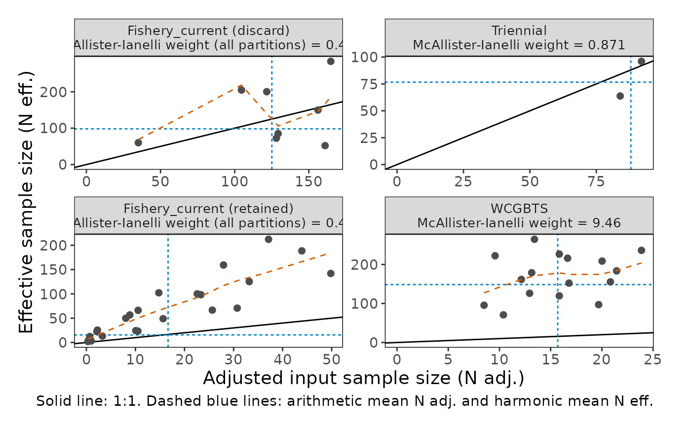
Each panel shows a 1:1 line, a loess smoother (dashed red, when there are
more than six distinct input sample sizes), the arithmetic mean of the
input sample sizes (vertical dashed line), and the harmonic mean of the
effective sample sizes (horizontal dashed line). The ratio of the harmonic
mean effective sample size to the mean input sample size, the
McAllister-Ianelli weight, is included in each panel label. Ratios below
one suggest that input sample sizes are too large relative to the fit. As
in Stock Synthesis, the weight is calculated across all partitions of a
fleet; multiplying it by the current variance adjustment gives the
Recommend_var_adj reported by Stock Synthesis.
Effective sample sizes from this formula are not appropriate for compositions fit with a Dirichlet-multinomial likelihood.
Equivalent plots in other packages
r4ss: r4ss::SSplotComps() subplot 7 ("N-EffN
comparison").
References
McAllister, M.K., and Ianelli, J.N. (1997). Bayesian stock assessment using catch-age data and the sampling-importance resampling algorithm. Canadian Journal of Fisheries and Aquatic Sciences 54: 284-300.
Examples
plot_composition_samples(bigskate_lencomp)
 # Stock Synthesis output converted with convert_output()
plot_composition_samples(stockplotr::example_data, comp_type = "length")