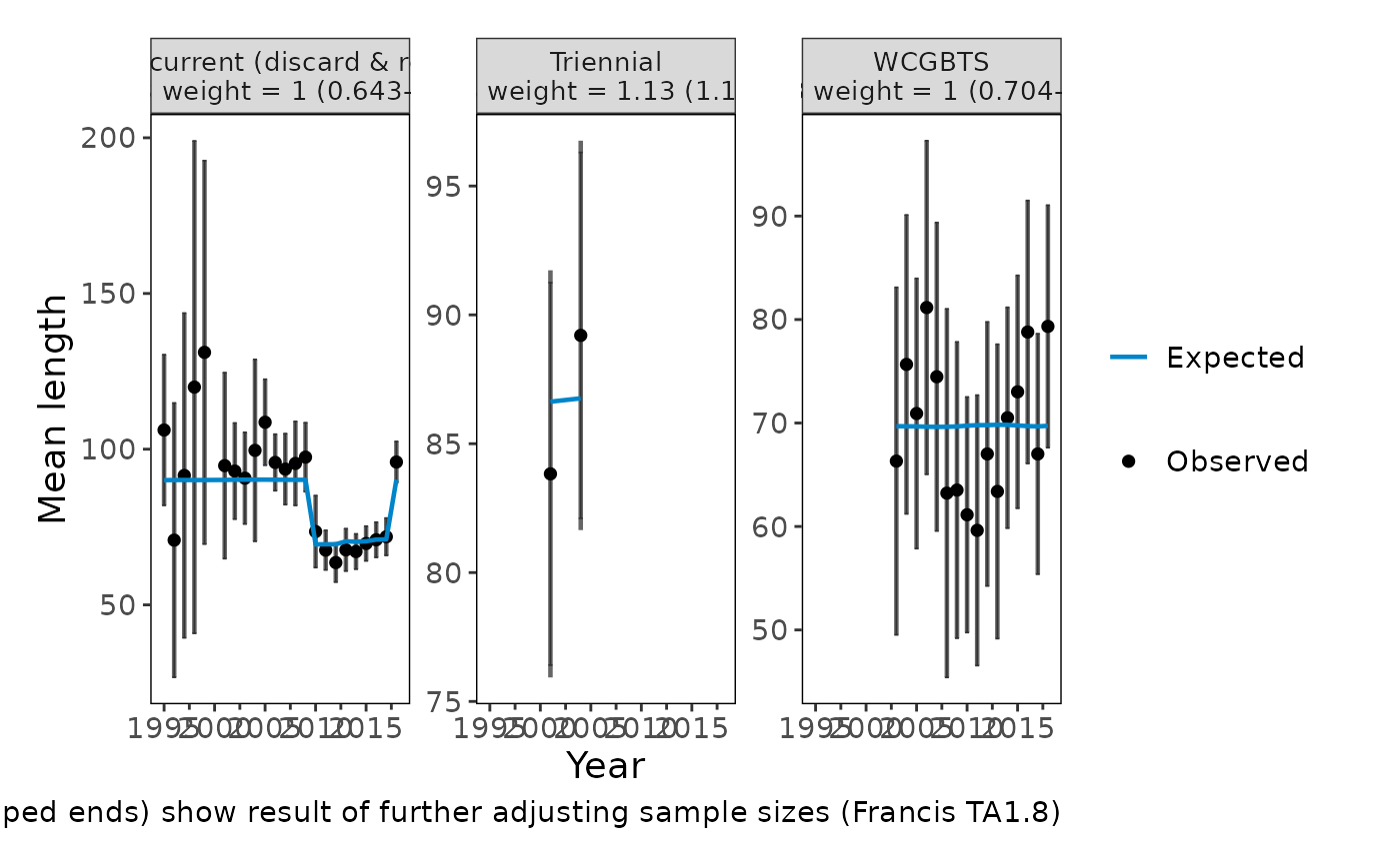
Plot mean age or length with Francis (method 8 in Table A1, TA1.8) data weights
Source:R/plot_composition.R
plot_composition_francis.RdTime series of the mean age or length in the observed and expected compositions. Developed as a diagnostic for the Francis (2011) data weighting method (TA1.8), the plot is also a useful summary of trends in compositions and lack of fit among years.
plot_composition_francis(
  dat,
  interval = 0.95,
  show_francis = TRUE,
  comp_type = NULL,
  fleet = NULL,
  ncol = NULL,
  direction = "v"
)
Arguments
- dat
A tibble returned from
convert_output()that contains composition data (see bigskate_lencomp), or composition data in any other format accepted byprepare_composition_data().- interval
Number. Coverage of the interval around the observed mean. Default: 0.95
- show_francis
Logical. TRUE/FALSE; add the Francis TA1.8 weight for each fleet to the panel label and show thinner, capped intervals representing sample sizes after applying that weight. Default: TRUE
- comp_type
String. Type of composition to keep when
datcontains more than one. Options: "age", "length", or NULL (keep all). Default: NULL- fleet
Character or numeric vector. Fleet(s) to keep, matching either the fleet name (e.g., "Fishery_current") or the fleet name with its partition (e.g., "Fishery_current (retained)"). NULL keeps all fleets. Default: NULL
- ncol
Number. Number of facet columns. NULL lets
ggplot2choose. Default: NULL- direction
String. Order of the panels: "v" fills panels down each column and then across, so consecutive years are stacked vertically and cohorts are easier to follow from panel to panel; "h" fills panels across each row.
Default: "v"
Value
A ggplot2 object.
Details
For each year and fleet (with sexes combined), the observed mean is \(\bar{x}_o = \sum_b x_b o_b\) and the expected mean is \(\bar{x}_e = \sum_b x_b e_b\), where \(x_b\) is the bin and \(o_b\) and \(e_b\) are the observed and expected proportions. Assuming a multinomial distribution, the standard error of the mean is \(\sqrt{v_e / N}\), where \(v_e = \sum_b x_b^2 e_b - \bar{x}_e^2\) is the variance of the expected composition and \(N\) is the sample size. Intervals are drawn around the observed means.
The Francis weight is \(1 / \mathrm{var}(r)\) where
\(r = (\bar{x}_o - \bar{x}_e) / SE\) are the standardized residuals of
the mean across years. As in Stock Synthesis and
r4ss::SSMethod.TA1.8(), all partitions of a fleet (e.g., retained and
discarded) share one weight, and its 95% interval is calculated by
bootstrapping the standardized residuals (1000 resamples), so use
set.seed() for reproducible intervals. The weight assumes a multinomial likelihood and has not been
adapted for Dirichlet-multinomial or other likelihoods.
Without expected values, only the observed means are plotted. Without sample sizes, no intervals or weights are shown.
Equivalent plots in other packages
r4ss: r4ss::SSplotComps() subplots 8 and 9, which
use r4ss::SSMethod.TA1.8().
References
Francis, R.I.C.C. (2011). Data weighting in statistical fisheries stock assessment models. Canadian Journal of Fisheries and Aquatic Sciences 68: 1124-1138.
Examples
plot_composition_francis(bigskate_lencomp)