Plot the distribution of composition residuals
Source:R/plot_composition_diagnostics.R
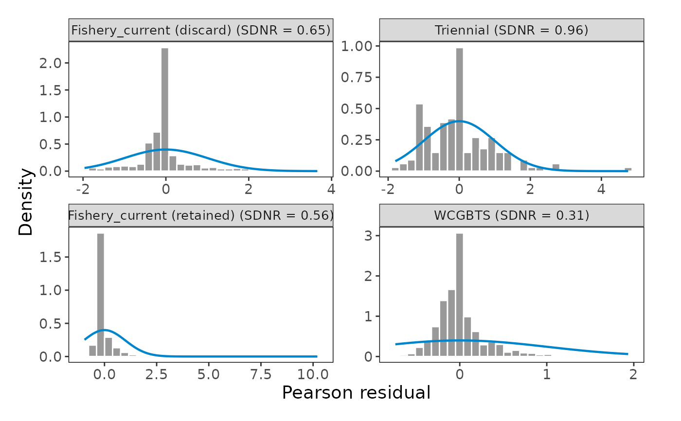
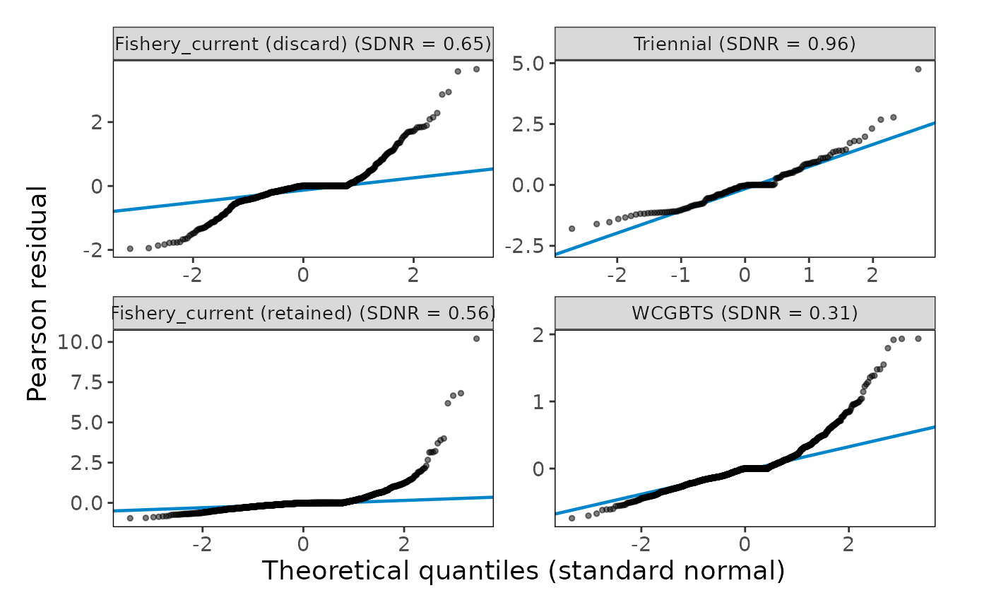
plot_composition_residual_distribution.RdQuantile-quantile plot or histogram of Pearson residuals for each fleet, to check for heavy tails, skewness, and outliers.
plot_composition_residual_distribution(
  dat,
  type = c("qq", "histogram"),
  comp_type = NULL,
  fleet = NULL,
  ncol = NULL,
  direction = "v"
)
Arguments
- dat
A tibble returned from
convert_output()that contains composition data (see bigskate_lencomp), or composition data in any other format accepted byprepare_composition_data().- type
String. Type of plot. Options: "qq" (normal quantile-quantile plot) or "histogram" (with a standard normal density overlaid). Default: "qq"
- comp_type
String. Type of composition to keep when
datcontains more than one. Options: "age", "length", or NULL (keep all). Default: NULL- fleet
Character or numeric vector. Fleet(s) to keep, matching either the fleet name (e.g., "Fishery_current") or the fleet name with its partition (e.g., "Fishery_current (retained)"). NULL keeps all fleets. Default: NULL
- ncol
Number. Number of facet columns. NULL lets
ggplot2choose. Default: NULL- direction
String. Order of the panels: "v" fills panels down each column and then across, so consecutive years are stacked vertically and cohorts are easier to follow from panel to panel; "h" fills panels across each row.
Default: "v"
Value
A ggplot2 object.
Details
The standard deviation of the normalized residuals (SDNR) for each fleet is included in the panel label. Values well above one suggest that the compositions are given more weight (larger sample sizes) than the fit supports. Pearson residuals for compositions are not expected to be exactly normally distributed, especially for bins with small expected proportions or small sample sizes, so treat departures in the tails with some caution.
See also
Examples
plot_composition_residual_distribution(bigskate_lencomp)
 plot_composition_residual_distribution(bigskate_lencomp, type = "histogram")