OSA Tutorial

Andrea Havron

2025-06-25

One-step ahead residuals introduction

Outline of methods and assumptions

Methods

Examples will reply on two models from the TMB example suite:

• simple.cpp: normal linear mixed model
• arxar1.cpp: generalized linear mixed model with separable covariance on lattice with AR1 structure in each direction

Examples can be run in R using: TMB::runExample(name = "simple") and TMB::runExample(name = "ar1xar1")

Assumption #1: Data and random effects are approximately normal

path <- here::here()
TMB::runExample(name = "randomwalkvalidation", exfolder = paste0(path,"/inst/examples"))

#Plot data: 
plot(1:length(Y), Y)

Full Guassian

#Correct Model
osa <- TMB::oneStepPredict(obj1, observation.name = "y", method = "fullGaussian")

qqnorm(osa$residual)
abline(0,1)

#Mis-specified Model
osa <- TMB::oneStepPredict(obj0, observation.name = "y", method = "fullGaussian")

qqnorm(osa$residual)
abline(0,1)

one-step Guassian

osa <- TMB::oneStepPredict(obj1, observation.name = "y", data.term.indicator = "keep", 
                      method = "oneStepGaussian")

qqnorm(osa$residual)
abline(0,1)

Assumption #2: Data are not approximately normal but have a defined cdf

#Plot data: 
ggplot2::ggplot(d, ggplot2::aes(x,y,fill = N)) + ggplot2::geom_raster()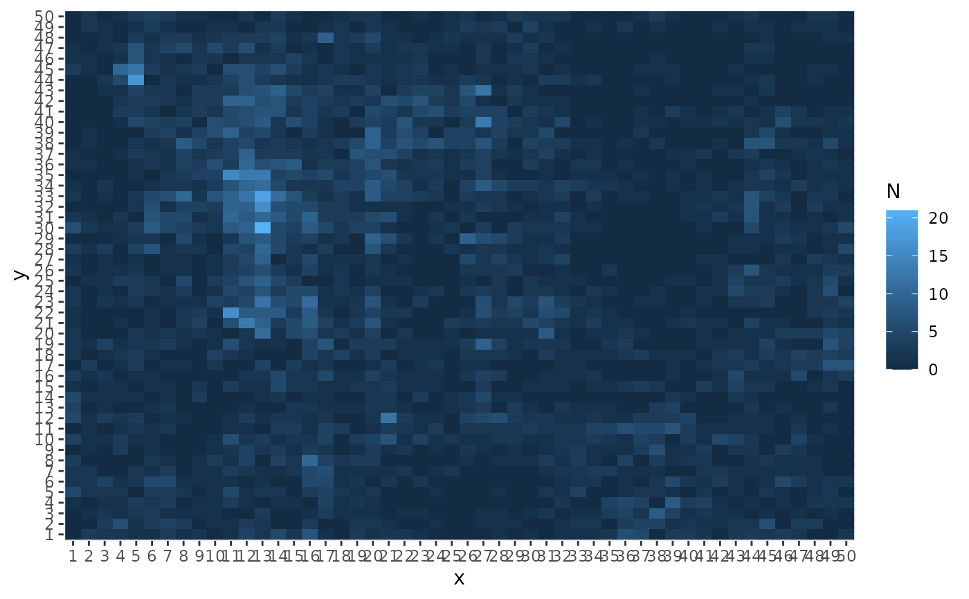

Data are discrete, so need to set discrete = TRUE

cdf

qqnorm(osa$residual);abline(0,1)

Assumption #3: Data are not approximately normal and do not have a defined cdf

qqnorm(osa$residual);abline(0,1)