Notes on Richards growth in Stock Synthesis

Author

Arni Magnusson and Ian Taylor

Introduction

The equations used in the Stock Synthesis implementation of the Richards curve, as found in the ADMB source code, are different from the equations in the Stock Synthesis User Manual (Methot et al. 2024). This vignette (1) shows that the equations are equivalent and (2) demonstrates the various shapes of the Richards curve using different values for the \(k\) and \(b\) parameters.

Methods

Install and load the r4ss package, so we can import Stock Synthesis model output.

remotes::install_github("r4ss/r4ss")
library(r4ss)

Parameter definitions

The Richards growth model has four parameters:

\(L_1\): length at age \(A_1\)
\(L_2\): length at age \(A_2\)
\(k\): growth coefficient
\(b\): shape parameter

and three input variables:

\(t\): age
\(A_1\): young age selected by user, for the estimation of \(L_1\)
\(A_2\): old age selected by user, for the estimation of \(L_2\)

SS3 Code

The following R function replicates the Richards growth implementation from the Stock Synthesis ADMB source code.

ss3_code <- function(t, L1, L2, k, b, A1, A2)
{
  LminR <- L1^b
  LmaxR <- L2^b
  LinfR <- LminR + (LmaxR - LminR) / (1 - exp(-k*(A2-A1)))
  temp <- LinfR + (LminR - LinfR) * exp(-k*(t-A1))
  temp^(1/b)
}

Schnute

The Schnute parametrization of the Richards curve is from Schnute (1981) (Eq. 15, case 1).

schnute <- function(t, L1, L2, k, b, A1, A2)
{
  (L1^b + (L2^b-L1^b) * (1-exp(-k*(t-A1))) / (1-exp(-k*(A2-A1))))^(1/b)
}

von Bertalanffy

The reparametrized von Bertalanffy function is from Schnute and Fournier (1980) (Eq. 7).

von_bertalanffy <- function(t, L1, L2, k, A1, A2)
{
  L1 + (L2-L1) * (1-exp(-k*(t-A1))) / (1-exp(-k*(A2-A1)))
}

Gompertz

Finally, a standard Gompertz function is found in Schnute (1981) (Eq. 2).

gompertz <- function(t, Linf, tau)
{
  Linf * exp(-exp(-k*(t-tau)))
}

Results

Stock Synthesis model output

Read estimated growth parameters from a fitted Stock Synthesis model.

# dir = the file path to the directory above where the example files are downloaded
model <- r4ss::SS_output(file.path(dir, "simple_small_richards"))
A1 <- subset(model$Growth_Parameters, Sex==1, A1, drop=TRUE)
A2 <- subset(model$Growth_Parameters, Sex==1, A2, drop=TRUE)
L1 <- subset(model$Growth_Parameters, Sex==1, L_a_A1, drop=TRUE)
L2 <- subset(model$Growth_Parameters, Sex==1, L_a_A2, drop=TRUE)
k <- subset(model$Growth_Parameters, Sex==1, K, drop=TRUE)
b <- model$parameters["Richards_Fem_GP_1", "Value"]
Linf <- subset(model$Growth_Parameters, Sex==1, Linf, drop=TRUE)

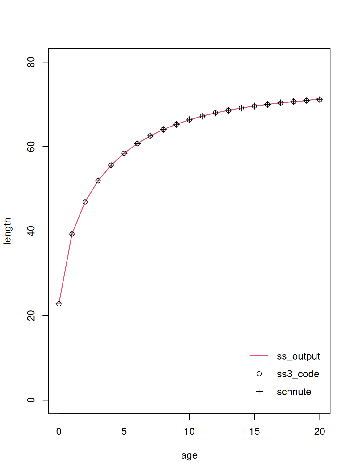
Compare three growth curves: length-at-age reported in the Stock Synthesis output, predicted lengths using the ss3_code() function, and predicted lengths using the schnute() function.

t <- 0:20
plot(Len_Beg~Age_Beg, model$endgrowth, subset=Sex==1, ylim=c(0,80),
     xlab="age", ylab="length", type="l", lwd=1.5, col=2)
points(t, ss3_code(t, L1, L2, k, b, A1, A2))
points(t, schnute(t, L1, L2, k, b, A1, A2), pch=3)
legend("bottomright", c("ss_output", "ss3_code", "schnute"),
       pch=c(NA, 1, 3), lty=c(1, NA, NA), lwd=c(1.5, NA, NA),
       col=c(2, 1, 1), bty="n", inset=0.02, y.intersp=1.5)

The predicted length from the ss3_code() and schnute() functions are in perfect agreement with each other. They are the same predicted lengths as reported in the Stock Synthesis output, except for the oldest age which is treated as a plus group inside the model, containing age 20 and older.

comparison <- data.frame(
  age = t,
  ss3_output = subset(model$endgrowth, Sex==1, Len_Beg, drop=TRUE),
  ss3_code = ss3_code(t, L1, L2, k, b, A1, A2),
  schnute = schnute(t, L1, L2, k, b, A1, A2)
)
print(comparison, row.names=FALSE)

 age ss3_output ss3_code  schnute
   0    22.7690 22.76900 22.76900
   1    39.3016 39.30161 39.30161
   2    46.8948 46.89477 46.89477
   3    51.9159 51.91588 51.91588
   4    55.5968 55.59675 55.59675
   5    58.4357 58.43566 58.43566
   6    60.6924 60.69238 60.69238
   7    62.5224 62.52241 62.52241
   8    64.0274 64.02738 64.02738
   9    65.2779 65.27789 65.27789
  10    66.3251 66.32514 66.32514
  11    67.2075 67.20754 67.20754
  12    67.9547 67.95467 67.95467
  13    68.5897 68.58973 68.58973
  14    69.1313 69.13126 69.13126
  15    69.5942 69.59425 69.59425
  16    69.9909 69.99095 69.99095
  17    70.3315 70.33147 70.33147
  18    70.6242 70.62422 70.62422
  19    70.8762 70.87622 70.87622
  20    71.3850 71.09338 71.09338

Special cases

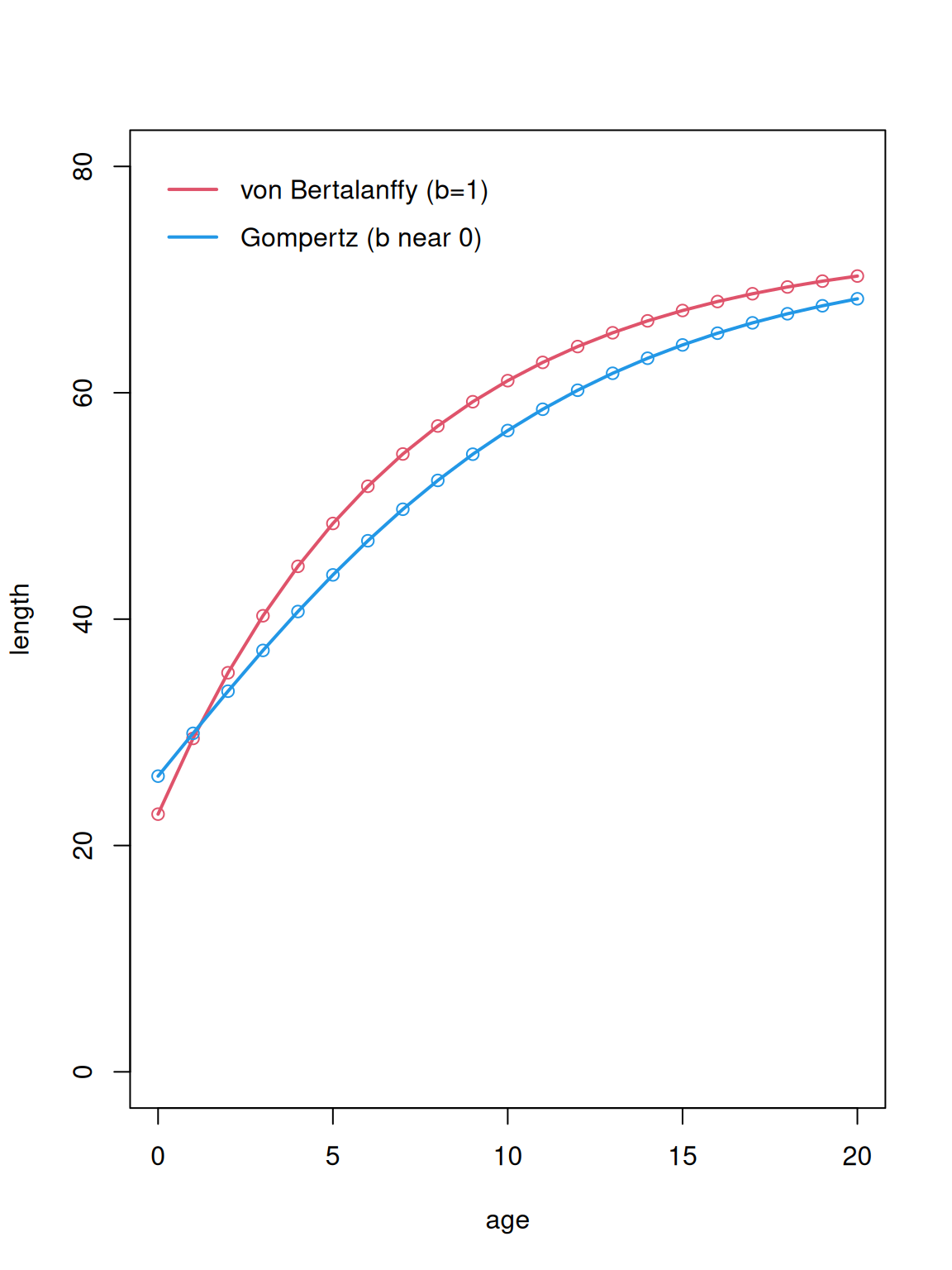
Special cases of the Richards curve include the von Bertalanffy (\(b\!=\!1\)) and Gompertz (\(b\!\to\!0\)) models. In the plot below, the lines are drawn using the actual von Bertalanffy and Gompertz functions, and the circles are drawn using the Richards curve with the appropriate values for the \(b\) parameter.

plot(NA, xlim=range(t), ylim=c(0,80), xlab="age", ylab="length")
lines(t, von_bertalanffy(t, L1, L2, k, A1, A2), ylim=c(0,80), lwd=2, col=2)
points(t, schnute(t, L1, L2, k, 1, A1, A2), col=2)
lines(t, gompertz(t, Linf, k), lwd=2, col=4)
Lg1 <- gompertz(A1, Linf, k)
Lg2 <- gompertz(A2, Linf, k)
points(t, schnute(t, Lg1, Lg2, k, 0.0001, A1, A2), col=4)
legend("topleft", c("von Bertalanffy (b=1)","Gompertz (b near 0)"),
       lwd=2, col=c(2,4), bty="n", inset=0.02, y.intersp=1.5)

Richards growth curves with different \(k\) and \(b\) combinations

x <- seq(0, 20, by=0.1)
L1 <- 5
L2 <- 80
A1 <- 0
A2 <- 20

plot(NA, xlim=range(x), ylim=c(0, 80), xlab="age", ylab="length")
z <- rich.colors.short(6)

lines(x, schnute(x, L1, L2, k=0.8,    b=-3,     A1, A2), lwd=2, col=z[1])
lines(x, schnute(x, L1, L2, k=0.8,    b=-2,     A1, A2), lwd=2, col=z[1])
lines(x, schnute(x, L1, L2, k=0.8,    b=-1,     A1, A2), lwd=2, col=z[1])
lines(x, schnute(x, L1, L2, k=0.4,    b=-1,     A1, A2), lwd=2, col=z[1])
lines(x, schnute(x, L1, L2, k=0.4,    b=0.0001, A1, A2), lwd=2, col=z[2])
lines(x, schnute(x, L1, L2, k=0.2,    b=0.0001, A1, A2), lwd=2, col=z[2])
lines(x, schnute(x, L1, L2, k=0.4,    b=1,      A1, A2), lwd=2, col=z[3])
lines(x, schnute(x, L1, L2, k=0.2,    b=1,      A1, A2), lwd=2, col=z[3])
lines(x, schnute(x, L1, L2, k=0.1,    b=1,      A1, A2), lwd=2, col=z[3])
lines(x, schnute(x, L1, L2, k=0.2,    b=2,      A1, A2), lwd=2, col=z[4])
lines(x, schnute(x, L1, L2, k=0.1,    b=2,      A1, A2), lwd=2, col=z[4])
lines(x, schnute(x, L1, L2, k=0.0001, b=2,      A1, A2), lwd=2, col=z[4])
lines(x, schnute(x, L1, L2, k=0.2,    b=3,      A1, A2), lwd=2, col=z[5])
lines(x, schnute(x, L1, L2, k=0.1,    b=3,      A1, A2), lwd=2, col=z[5])
lines(x, schnute(x, L1, L2, k=0.0001, b=3,      A1, A2), lwd=2, col=z[5])
lines(x, schnute(x, L1, L2, k=0.1,    b=4,      A1, A2), lwd=2, col=z[6])
lines(x, schnute(x, L1, L2, k=0.0001, b=4,      A1, A2), lwd=2, col=z[6])
lines(x, schnute(x, L1, L2, k=0.0001, b=5,      A1, A2), lwd=2, col=z[6])
lines(x, schnute(x, L1, L2, k=0.0001, b=6,      A1, A2), lwd=2, col=z[6])

legend("bottomright", c("b: 4 to 6", "b: 3", "b: 2", "b: 1", "b: 0.001",
       "b: -1 to -3"), lwd=2.5, col=rev(z), bty="n", inset=0.02, y.intersp=1.2)

Discussion

Range of permissible \(b\) values

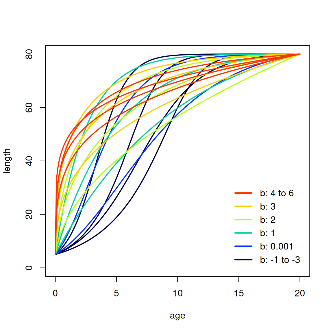
The Schnute parametrization of the Richards curve used in Stock Synthesis can produce a wide variety of shapes, based on the value of the \(b\) parameter, as demonstrated in Section 3.3. When \(A_1\) is greater than the youngest age in the model, some combinations of Richards growth parameters can lead to undefined (NaN) predicted length for the younger ages. The choice of \(A_1\) and \(A_2\) will affect the possible growth curve shapes.

The one value of \(b\) that is not allowed when using the Richards growth curve in Stock Synthesis is \(b\!=\!0\). This also holds for the R functions ss3_code() and schnute() used in this vignette. When estimating \(b\) as a floating-point number, there is effectively no risk of the parameter becoming precisely zero during estimation, as long as the initial value is non-zero. To use a Gompertz growth curve, the \(b\) parameter can be fixed at a small value such as 0.0001, as demonstrated in Section 3.2.

Proof of `ss3_code()` being equivalent to `schnute()`

The above demonstrations comparing the Stock Synthesis output, ss3_code() and schnute() indicate that they are mathematically equivalent, meaning that the same parameter input produces the same growth curve. The equivalence can also be proven algebraically.

In Stock Synthesis, the Richards growth curve is implemented as

ss3_code <- function(t, L1, L2, k, b, A1, A2)
{
  LminR <- L1^b
  LmaxR <- L2^b
  LinfR <- LminR + (LmaxR - LminR) / (1 - exp(-k*(A2-A1)))
  temp <- LinfR + (LminR - LinfR) * exp(-k*(t-A1))
  temp^(1/b)
}

\[ L_t ~=~ \Big[\,L_{\infty R} \;+\; (L_1^b-L_{\infty R})\, e^{-k(t-A_1)}\,\Big]^{1/b} \]

where:

\[L_{\infty R} ~=~ L_1^b \;+\; \frac{L_2^b\,-\,L_1^b}{1-e^{-k(A_2-A_1)}}\]

We proceed by replacing \(L_{\infty R}\) with its definition and then gradually simplify the equation:

\[\begin{eqnarray*} L_t &=& \bigg[\,L_1^b \;+\; \frac{L_2^b-L_1^b}{1-e^{-k(A_2-A_1)}} \;+\; \left(L_1^b\,-\,\Big[L_1^b \,+\, \frac{L_2^b-L_1^b}{1-e^{-k(A_2-A_1)}}\Big]\right) e^{-k(t-A_1)}\,\bigg]^{1/b}\\[4ex] L_t &=& \bigg[\,L_1^b \;+\; \frac{L_2^b-L_1^b}{1-e^{-k(A_2-A_1)}} \;+\; \left(L_1^b\,-\, L_1^b \,-\, \frac{L_2^b-L_1^b}{1-e^{-k(A_2-A_1)}} \right) e^{-k(t-A_1)}\,\bigg]^{1/b}\\[4ex] L_t &=& \bigg[\,L_1^b \;+\; \frac{L_2^b-L_1^b}{1-e^{-k(A_2-A_1)}} \;-\; \frac{L_2^b-L_1^b}{1-e^{-k(A_2-A_1)}}\, e^{-k(t-A_1)}\,\bigg]^{1/b}\\[4ex] L_t &=& \bigg[\,L_1^b \;+\; (L_2^b-L_1^b)\,\frac{1}{1-e^{-k(A_2-A_1)}} \;-\; (L_2^b-L_1^b)\,\frac{e^{-k(t-A_1)}}{1-e^{-k(A_2-A_1)}}\,\bigg]^{1/b}\\[4ex] L_t &=& \left[\:L_1^b\;+\;(L_2^b-L_1^b)\, \frac{1-e^{-k(t-A_1)}}{1-e^{-k(A_2-A_1)}}\,\right]^{1/b} \end{eqnarray*}\]

schnute <- function(t, L1, L2, k, b, A1, A2)
{
  (L1^b + (L2^b-L1^b) * (1-exp(-k*(t-A1))) / (1-exp(-k*(A2-A1))))^(1/b)
}

FSA package

The FSA package on CRAN (Ogle et al. 2023) is a useful reference to navigate through the plethora of alternative parametrizations of different growth curves. Among the FSA function calls that are relevant to this vignette are:

library(FSA)
Schnute(t, case=1, ...)
Schnute(t, case=2, ...)

Schnute case 1 (Schnute 1981, Eq. 15) is the same as schnute() used in this vignette.

Schnute case 2 (Schnute 1981, Eq. 16) is a Gompertz growth model parametrized with \(L_1\), \(L_2\), and \(k\), similar to ss3_code() and schnute() when \(b\) is fixed at nearly 0.

References

Methot, R. D., C. R. Wetzel, I. G. Taylor, K. L. Doering, E. F. Perl, and K. F. Johnson. 2024. Stock Synthesis User Manual Version 3.30.23. https://github.com/nmfs-ost/ss3-doc/releases/v3.30.23.

Ogle, Derek H., Jason C. Doll, A. Powell Wheeler, and Alexis Dinno. 2023. FSA: Simple Fisheries Stock Assessment Methods. https://CRAN.R-project.org/package=FSA.

Schnute, Jon. 1981. “A Versatile Growth Model with Statistically Stable Parameters.” Canadian Journal of Fisheries and Aquatic Sciences 38 (9): 1128–40. https://doi.org/10.1139/f81-153.

Schnute, Jon, and David Fournier. 1980. “A New Approach to Length–Frequency Analysis: Growth Structure.” Canadian Journal of Fisheries and Aquatic Sciences 37 (9): 1337–51. https://doi.org/10.1139/f80-172.