Testing palettes for color vision deficiency

Background

We are testing that the existing NMFS color palettes are usable to someone with color vision deficiency (C.V.D.).

We’ll use an R package called dichromat to approximate how these palettes might be perceived by someone with any of the most common forms of C.V.D.: protanopia, deutanopia, and tritanopia.

This analysis is based on this tutorial by Hannah Weller.

Install packages

install.packages("dichromat")
install.packages("recolorize")
install.packages("gridExtra")

Load libraries

library(dichromat)
library(recolorize)
library(gridExtra)

Create a function that shows perceptions of palettes

show_cvd_pals <- function(palette) {
  # Convert palette into three palettes approximating how someone with each type of C.V.D. would perceive the original palette

  ## protanopia
  protan <- dichromat::dichromat(palette, type = "protan")
  ## deutanopia
  deutan <- dichromat::dichromat(palette, type = "deutan")
  ## tritanopia
  tritan <- dichromat::dichromat(palette, type = "tritan")

  # Plot the palettes and compare
  layout(matrix(1:4, nrow = 4))
  par(mar = rep(1, 4))

  recolorize::plotColorPalette(palette, main = "Trichromacy ('normal color vision')")
  recolorize::plotColorPalette(protan, main = "Protanopia")
  recolorize::plotColorPalette(deutan, main = "Deutanopia")
  recolorize::plotColorPalette(tritan, main = "Tritanopia")
}

Test main palettes

# import main palettes from nmfs_cols.R file
core_nmfs_pals <- list(
  `oceans` = nmfs_cols("pale_sea_blue", "light_sea_blue", "processblue", "reflexblue", "national", "o50pblack"),
  `waves` = nmfs_cols("pale_teal", "bright_teal", "westcoast", "dark_teal_green"),
  `seagrass` = nmfs_cols("bright_seagrass", "ltgreen", "southeast", "dark_seagrass"),
  `urchin` = nmfs_cols("bright_urchin", "vivid_urchin", "midatlantic", "dark_urchin"),
  `crustacean` = nmfs_cols("bright_crustacean", "ltorange", "alaska", "dark_crustacean"),
  `coral` = nmfs_cols("bright_coral", "vivid_coral", "pacificislands", "dark_coral"),
  `regional` = nmfs_cols("national", "westcoast", "southeast", "midatlantic", "alaska", "pacificislands")
)

# Show comparisons for each palette
for (i in 1:length(core_nmfs_pals)) {
  print(paste0(names(core_nmfs_pals)[i], " palette"))
  show_cvd_pals(core_nmfs_pals[[i]])
}

## [1] "oceans palette"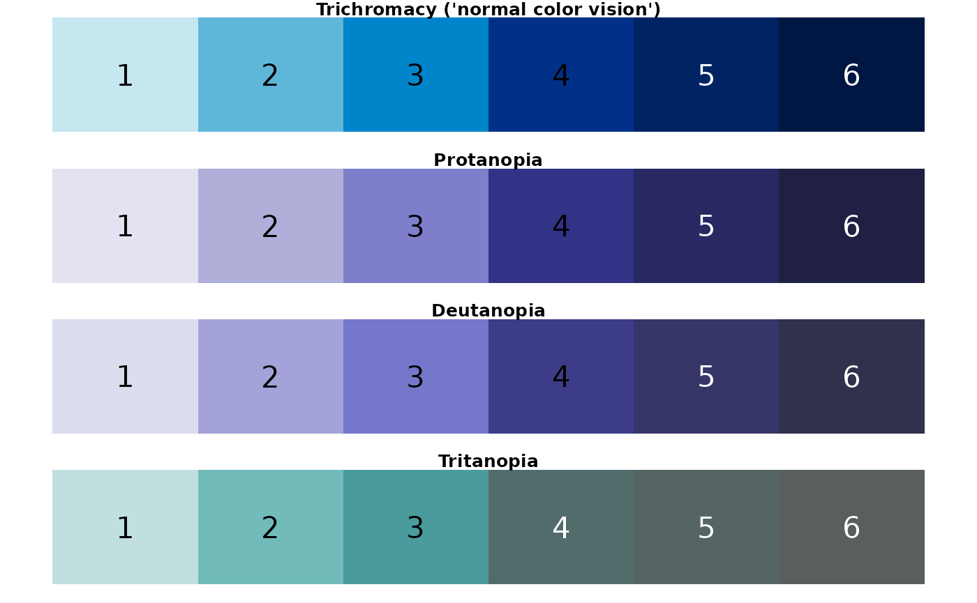

## [1] "waves palette"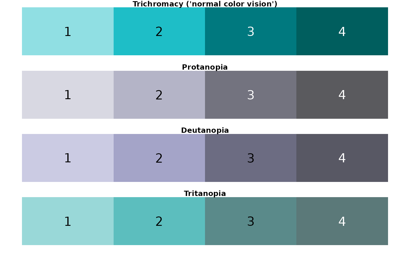

## [1] "seagrass palette"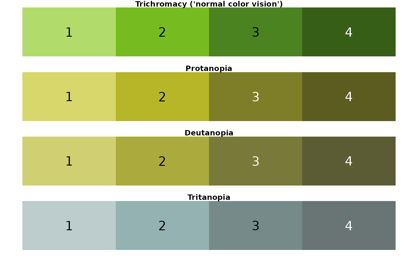

## [1] "urchin palette"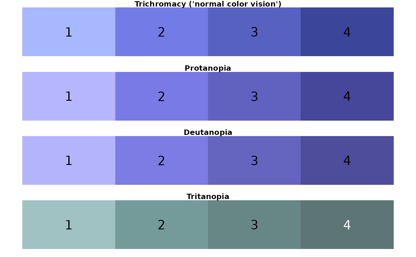

## [1] "crustacean palette"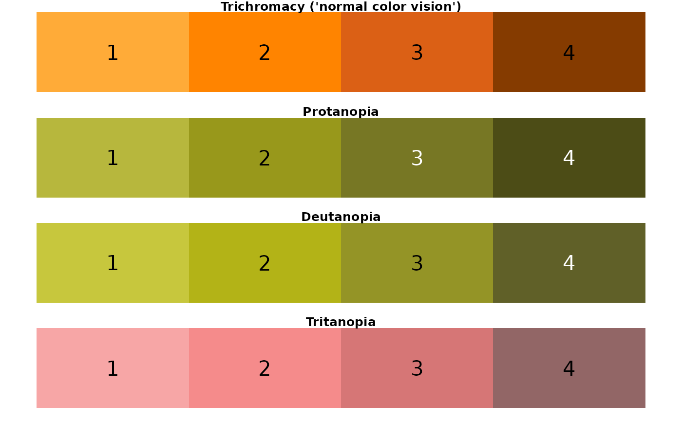

## [1] "coral palette"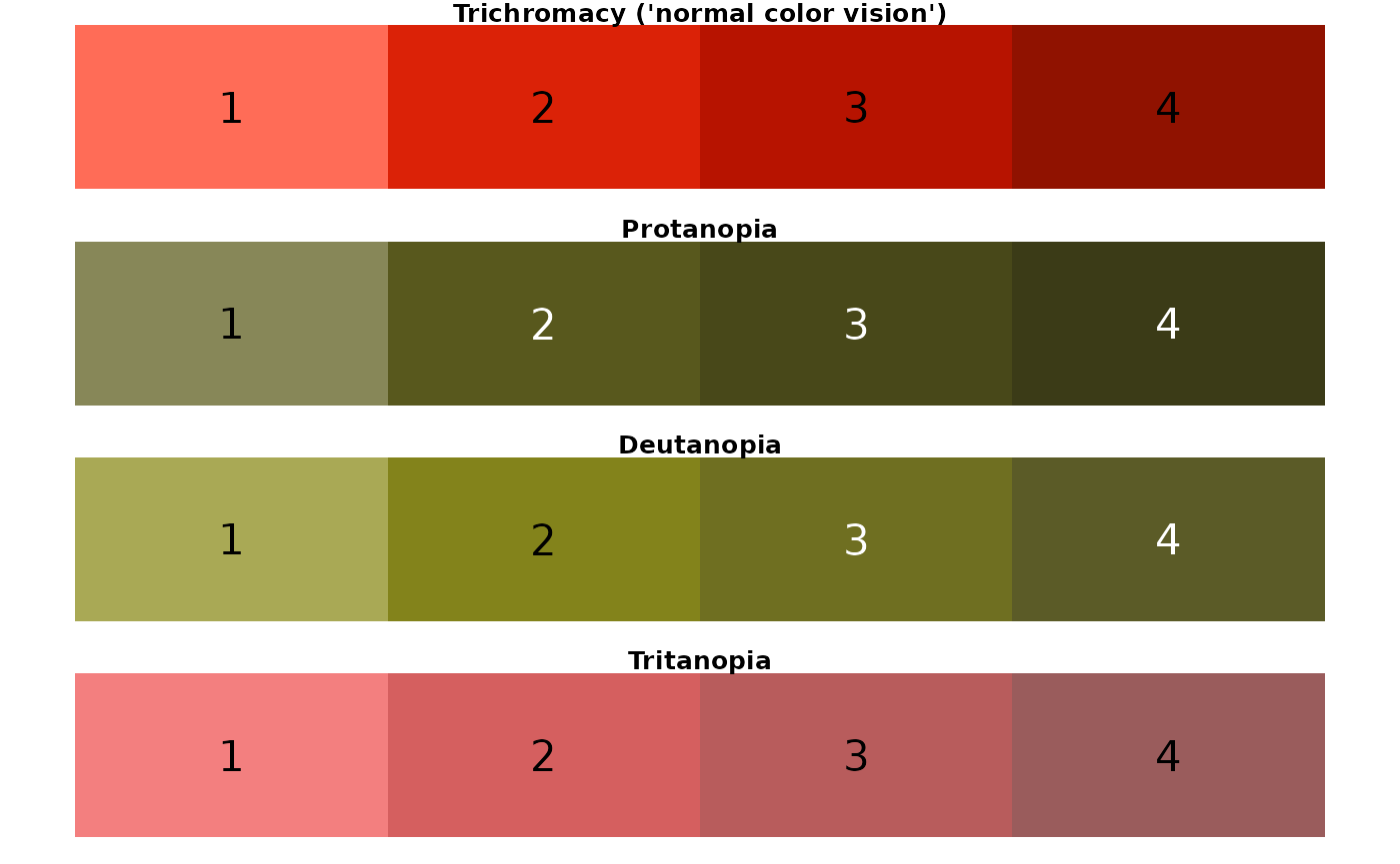

## [1] "regional palette"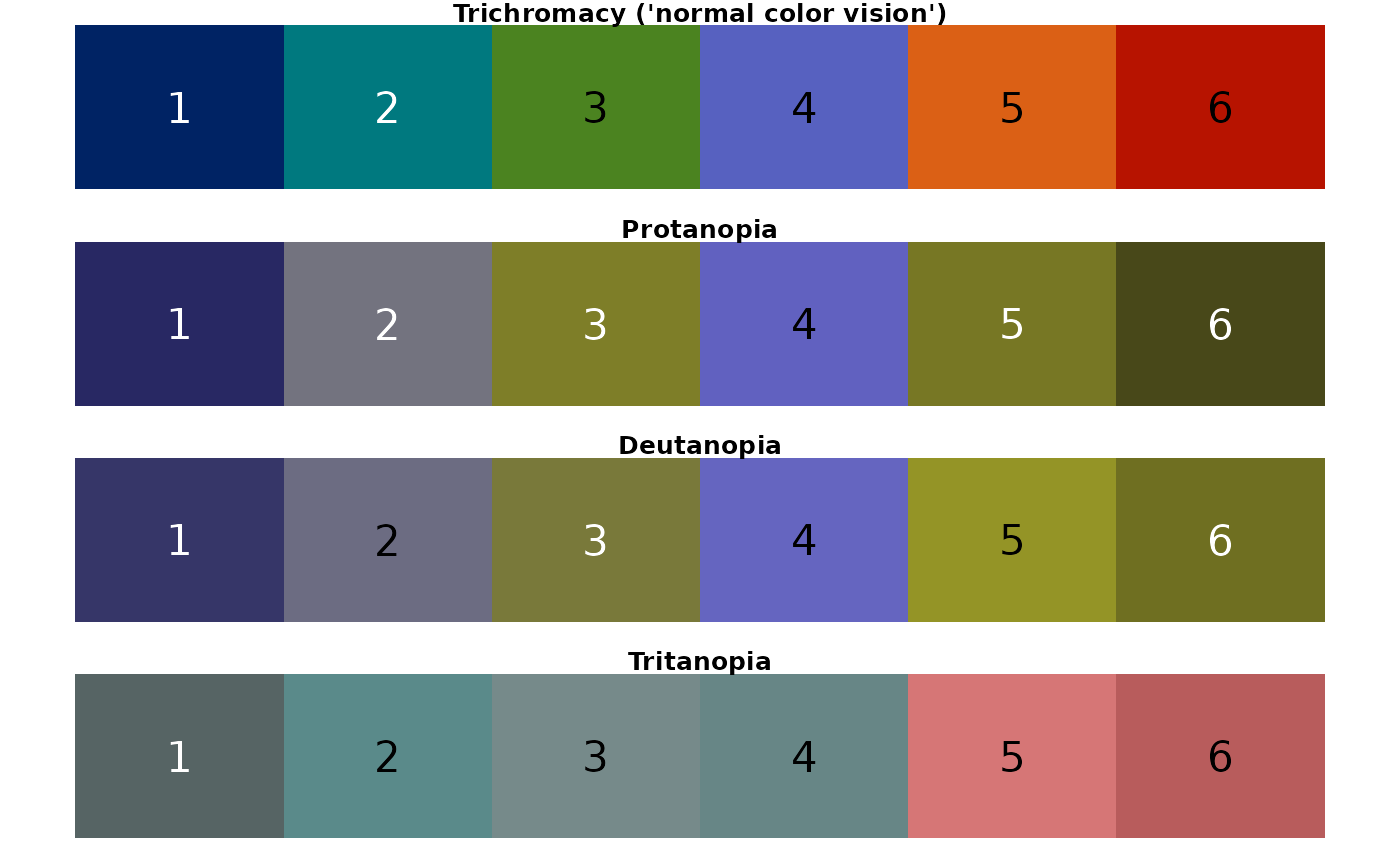

Conclusion: For someone with C.V.D., the regional palette could be challenging to discern. In particular, colors look very similar when viewed with the following perceptions: protanopia (3, 5); deutanopia (3, 5, 6); tritanopia (2, 3, 4).

Test alternative regional color palette

Create alternative palettes

# Option 1: using existing NMFS colors
regions_alt1 <- c(
  "#002364", # "national"
  "#00797F", # "westcoast"
  "#76BC21", # "ltgreen"
  "#5761C0", # "midatlantic"
  "#DB6015", # "alaska"
  "#B71300" # "pacificislands"
)

# Option 2: using some colors outside of the NMFS color set
regions_alt2 <- c(
  "#016080", # new color
  "#57aeb2", # new color
  "#26DC61", # new color
  "#8851D0", # new color
  "#DB6015", # "alaska"
  "#B71300" # "pacificislands"
)

alt_regional_pals <- list(
  `Alternative regional palette 1` = regions_alt1,
  `Alternative regional palette 2` = regions_alt2
)

Show alternative palettes

for (i in 1:length(alt_regional_pals)) {
  print(names(alt_regional_pals)[i])
  show_cvd_pals(alt_regional_pals[[i]])
}

## [1] "Alternative regional palette 1"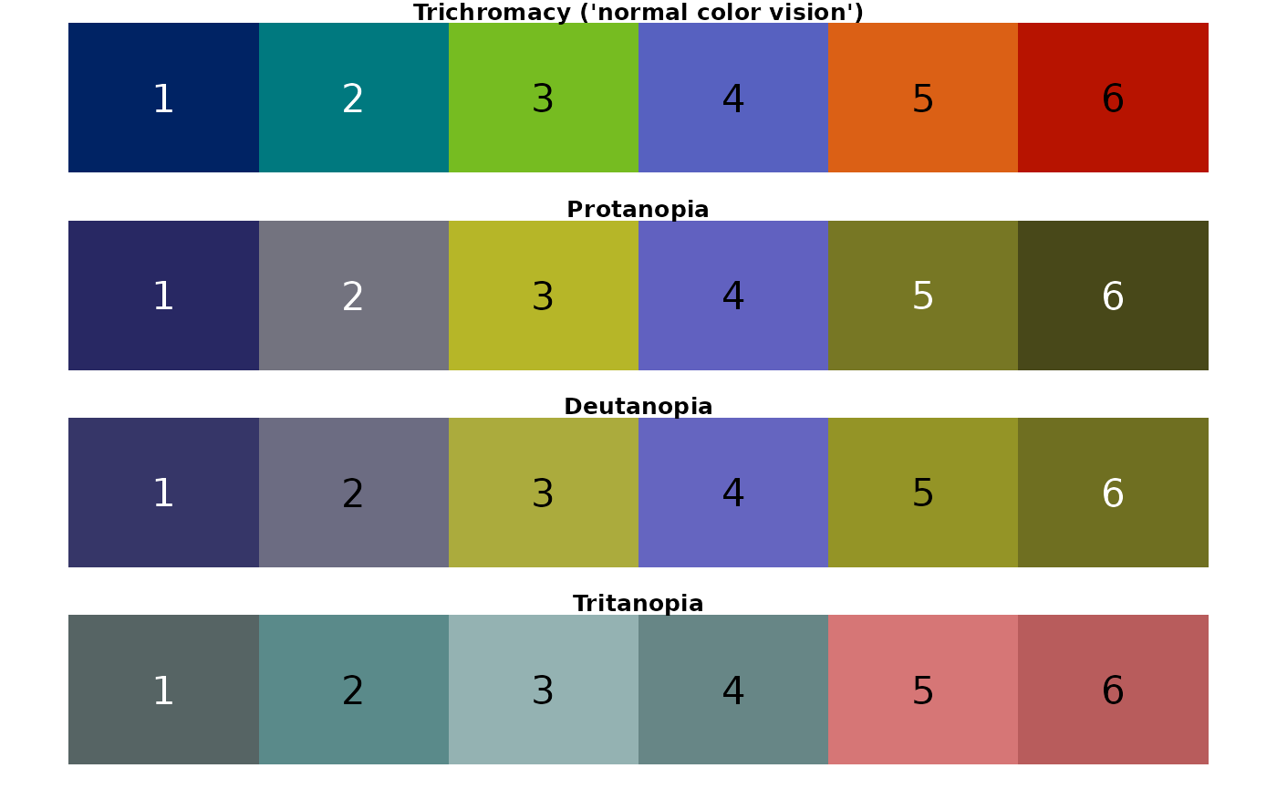

## [1] "Alternative regional palette 2"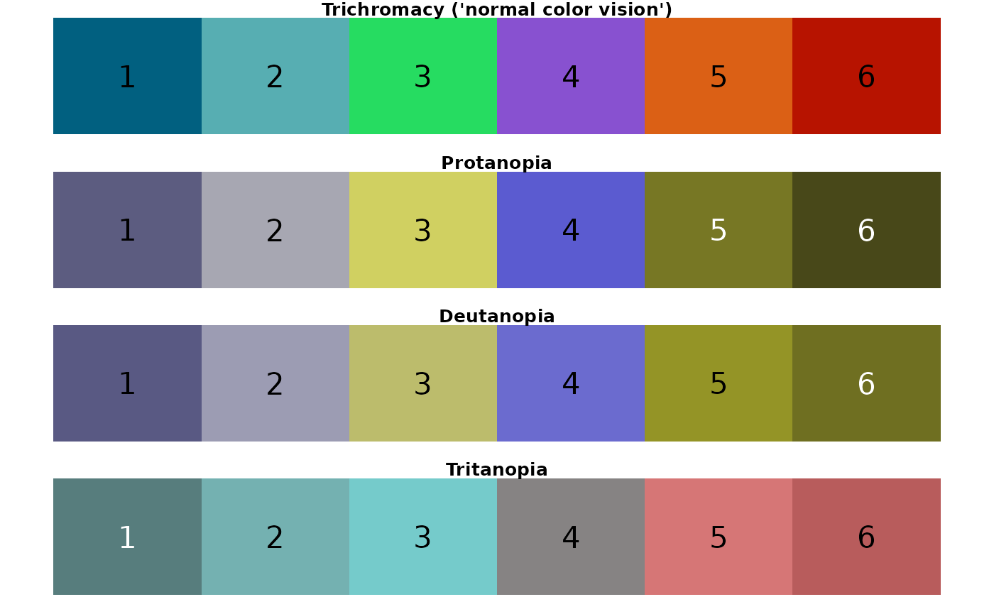

Show alternative palettes in figures

show_cvd_plots <- function(pal,
                           pal_name) {
  test_data <- data.frame(
    palette_color = c(
      "1", "2", "3", "4", "5", "6",
      "1", "2", "3", "4", "5", "6"
    ),
    y = c(
      1, 2, 3, 4, 5, 6,
      2, 3, 4, 5, 6, 7
    )
  )

  type <- "Trichromacy ('normal color vision')"
  orig <- ggplot2::ggplot(
    data = test_data,
    aes(
      x = palette_color,
      y = y,
      color = palette_color
    )
  ) +
    geom_point(
      size = 4,
      shape = 19
    ) +
    geom_line(size = 1) +
    theme_light() +
    theme(legend.position = "none") +
    labs(
      subtitle = type,
      x = "Palette color"
    ) +
    scale_color_manual(values = pal)
  orig

  type <- "Protanopia"
  protan <- orig +
    labs(subtitle = type) +
    scale_color_manual(values = dichromat::dichromat(pal, type = "protan"))
  protan

  type <- "Deutanopia"
  deutan <- orig +
    labs(subtitle = type) +
    scale_color_manual(values = dichromat::dichromat(pal, type = "deutan"))
  deutan

  type <- "Tritanopia"
  tritan <- orig +
    labs(subtitle = type) +
    scale_color_manual(values = dichromat::dichromat(pal, type = "tritan"))
  tritan

  four_plots <- gridExtra::grid.arrange(orig, protan, deutan, tritan,
    top = pal_name
  )

  return(four_plots)
}

for (i in 1:length(alt_regional_pals)) {
  show_cvd_plots(
    pal = alt_regional_pals[[i]],
    pal_name = names(alt_regional_pals)[i]
  )
}

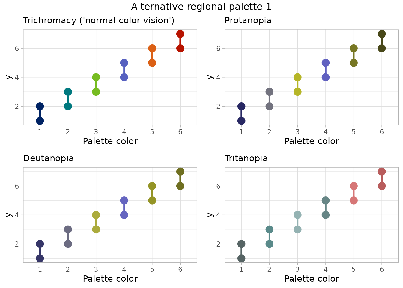
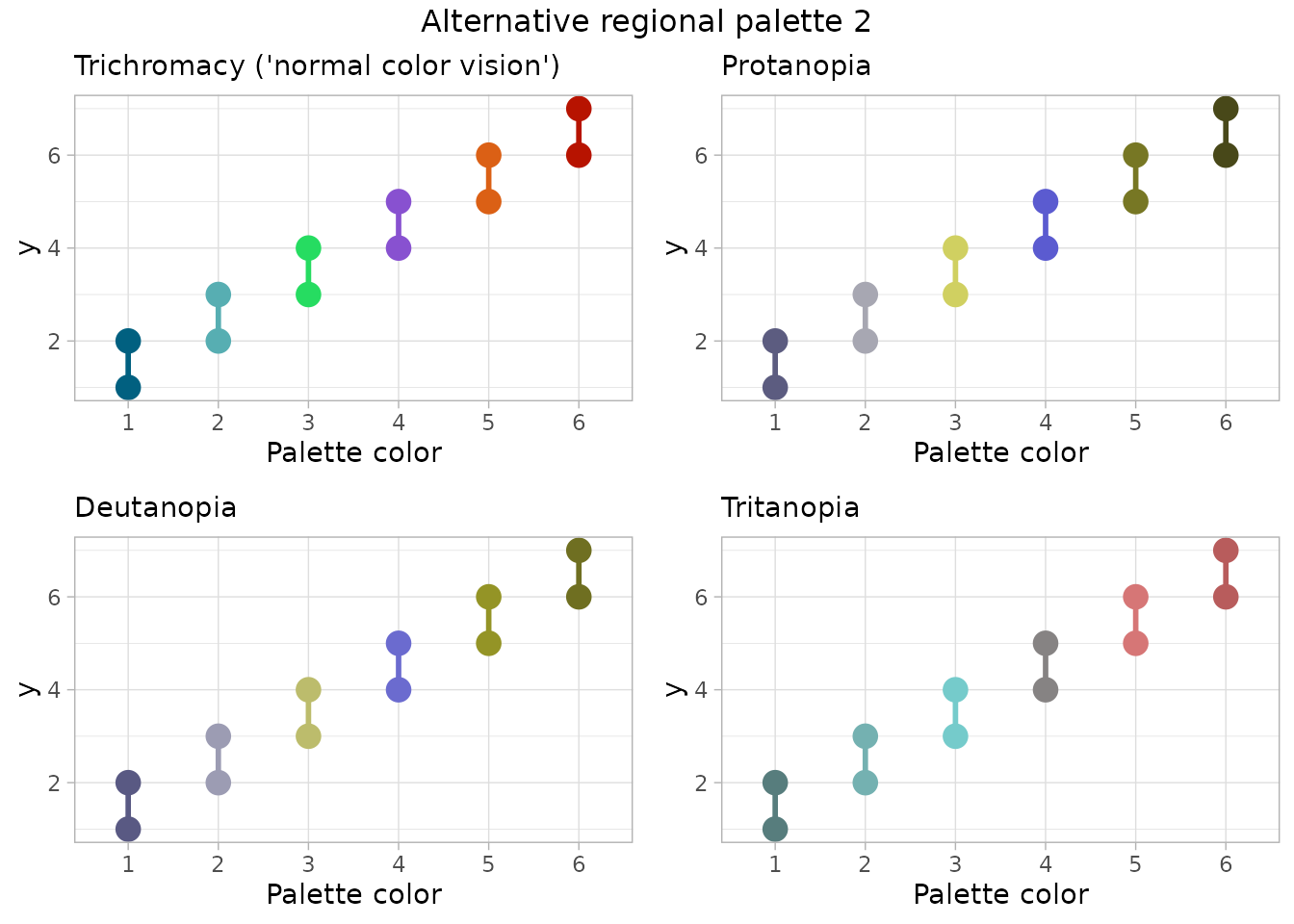
Conclusion: For someone with C.V.D., the alternative palette 1 shows colors 2 & 4 as very similar for tritanopia. Alternative palette 2 provides colors that seem distinguishable for all types of color perception, but multiple colors in this palette are outside the NMFS brand color set.

Both alternative regional palettes (“regional_alt1” and “regional_alt2”, respectively) are available in the package.

display_nmfs_palette("regional_alt1", 6)

display_nmfs_palette("regional_alt2", 6)